1 Introduction
In the past several years, deep learning methods based on artificial neural networks have revolutionized the analysis of speech, text and images [1,2]. The individual breakthroughs in language and vision have led naturally to the confrontation of a variety of tasks that combine these two modalities. Video captioning, as captured in the MSR-VTT Challenge [3] Fig. 1 is one of the major applications of the combination of visual and language modalities. Datasets with multiple modalities are of increasing importance for machine learning since they broaden the space of available labelled instances. For Konica Minolta areas like image and text or video and audio are applications where multiple modalities come into play. In particular, benefiting from the advances in the Natural Language Processing (NLP) and Computer Vision (CV) research communities, video captioning as shown in Fig. 2 has rapidly attracted increasing attention over a short period of time and developed in a variety of directions.
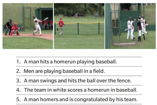
Fig. 1 Example of labelled MSRVTT video clip. The clip is typically 5 seconds long. Each clip has five captions generated by human beings.
In contrast to image captioning, video captioning is substantially more challenging due to the need to (a) ingest much more data, and (b) capture action (verbs) rather than focusing primarily on objects (nouns) with a presumed relationship.
In general, video action understanding is a difficult and challenging task and accurate video action understanding can provide many benefits in several business domains, such as, security, manufacturing, and retails.
Video captioning is one step towards accurate video action understanding and predication. Many models have been developed which differ depending on the precise task being addressed; for example, writing a caption for a given a video as opposed to choosing a caption from a list that best matches with a given video. One unifying feature of most video-text models, however, is the positing of an abstract joint space into (and out of) which the video and the language are encoded (decoded). Indeed, the encoding process can be considered as a problem all its own.
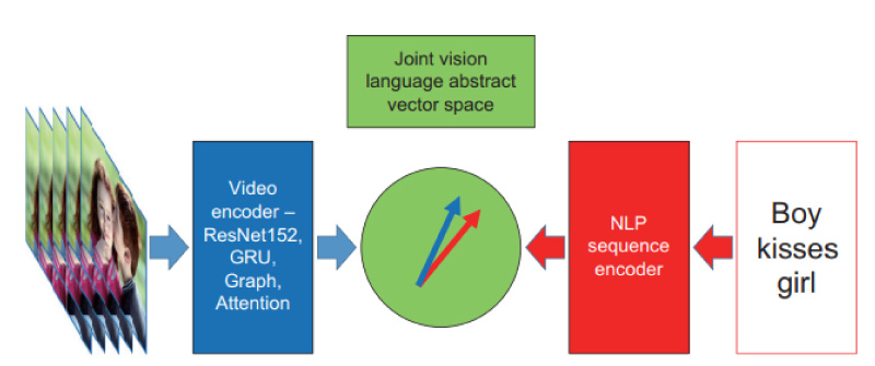
Fig. 2 Video to text machine learning requires that both images and language be encoded into a shared abstract space. Comparison of the projected vectors is then trained against ground truth to align the embeddings from the two modalities.
2 Graph neural network
In that context a recently developed technique – typified in a paper by Li et al [3] on which we will focus in this technical report – is to employ feature graphs to aid in the encoding of a video. Such a graph consists of nodes and edges, in symbols G=(N,E). For these graphs the nodes are vectors representing the features extracted from the graph and the edges are learned relationships between those features, which we discuss in greater detail below.
The primary function of the graph is to employ an algorithm called the graph convolutional neural network (GCN) [4,5] in order to pass information between the nodes – the expectation being that this provides a better representation of the whole video.
GCNs perform similar operations to convolutional neural networks (CNNs) where the model learns the features by inspecting neighboring nodes. The major difference between CNNs and GCNs is that CNNs are specially built to operate on regular (Euclidean) structured data, while GCNs are the generalized version of CNNs where the numbers of node connections vary and the nodes are unordered (irregular on nonEuclidean structured data).
Konica Minolta Labs U.S A has open innovation research project with Professor Raymond Fu of Northeastern University. The topic of the first year of that program was video captioning and the group produced algorithms and code that established stateof-the-art results in the MSRVTT challenge [3] on matching videos and captions. The architecture of that model is shown in Fig. 3.
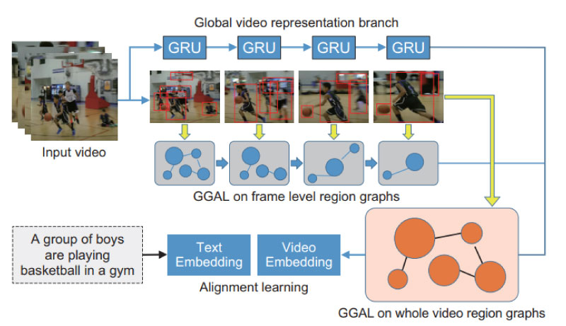
Fig. 3 Overview of the GGAL architecture, emphasizing the video encoding branch. Two kinds of graph are constructed: a frame level graph and a global graph. The global graph is created from faster R-CNN features and is analyzed in this paper.
2. 1 Graph guided attention learning
Here, we want to simply present an overview of the NEU developed model, Guided Graph Attention Learning (GGAL) enhances the video learning by capturing important region-level semantic concepts within the video. The inputs to the model are a series of videos (typically about five seconds in length) and, for each video, ten captions that have been generated by human beings. The objective is, upon training, to input either a video or a caption and to infer the correct caption or video.
In this paper we are specifically interested in the encoding of the video (as opposed to the text encoding function, see Fig. 3). In deep learning it is common to encode sequential data with a recurrent neural network. A video is an interesting case because it contains visual data in each frame but then the frames themselves form a sequence. The solution is to first extract ImageNet pre-trained features from each RGB frame using ResNet-152. The resulting sequence of frame-level scene features are:
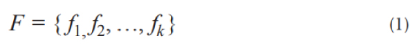
where fi ∈RD and D is a hyperparameter (typically 2048). The number of frames, typically 20, is denoted k. These features are then fed into a gated recurrent unit (GRU) to learn the sequential properties of the action.
At the same time, the frames are analyzed for framelevel features using a region-of-interest algorithm such as Faster R-CNN (here using ResNet-101 as a backbone). In this case, every frame i contains a finite set of features which we denote:
where again ri j ∈RD and there are n features extracted for each frame. In the work cited here there are generally n=25 features per frame.
Note that in the GGAL model there are two sets of feature and thus two types of graphs. In the first case, each frame is cast as a graph based on the scene features which are encoded in one vector per frame, fi. In the second case, one global graph is constructed from the faster R-CNN extracted regions of interest and associated features. It is this second graph, and the graph convolutional neural network that is applied to it, that we focus on in the remainder of this report.
2. 2 Region features as a graph
In any video the features which can be discerned in each frame are not isolated but have some relationship with each other. This relationship can be semantic (e.g. a boy kicks a ball suggests that a feature for boy and a feature for ball are related). The relationship can be frame-to-frame (the same ball at successive times), or it can also be just physical proximity within a frame. These kinds of relationships between a collection of entities – or nodes – are the essence of graphs, and the relationships themselves are manifested as edges between the nodes.
For this case the set of vectors R are treated as the features of a set of N =n∙k nodes. The edges between these nodes are learned parameters. Specifically, if we denote the edges between ri and rj (for notational simplicity we will now use only one index on each feature which range from 1 to N =n∙k) as A(ri , rj)= wϕ(ri)∙wϑ(rj) then the composite functions are simply fully connected layers, that is: wϕ(rj)=Wϕ∙rj and wϑ(rj) = Wϑ∙rj. The weight matrices Wϕ and Wϑ are learned during training.
As shown in the model architecture in Fig. 3, we perform a Graph Convolutional Network (GCN) operation[4] to learn relationship enhanced region features by message passing on this fully-connected region graph. Response of each node is computed based on the message passing with its neighbors defined by the graph relations. We add residual connections to the original GCN to help the training:

Where Wg is a weight matrix of the GCN layer with dimension D×D, Wr is the weight matrix of the residual structure. A is the above-mentioned edge (also called “affinity”) matrix. The output Rw′ = {r1′,r2′…,rN′}, ri′ ∈R D is the semantic relationship enhanced representation for the region nodes.
The meaning of Equation (3) can be readily understood by referring to Fig. 4. Each node has a 2048- dimension feature vector ri. The affinity matrix A, multiplying the feature vector, produces a linear combination of neighboring node feature vector weighted by the strength of the relevant edges. In the illustration in Fig. 4 we represent the feature vectors by the colors of the nodes. After one GCN step, those nodes with strong connections have had their colors mixed, e.g. a blue node strongly connected to a red node has caused both nodes to change to purple. Similarly, red and yellow nodes become orange.
The GCN mixing can be applied only once or it can be applied several times. The choice here is entirely empirical and the objective is simply to produce a set of node feature vectors that share information and (hopefully) make a better encoding of the video.
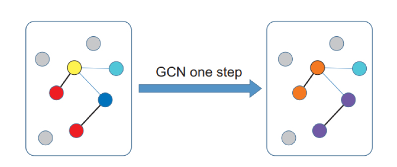
Fig. 4 Illustration of the graph convolutional neural network process. Nodes with features – illustrated by the colors – are connected by edges. The GCN step then mixes the features between nodes according to their connections.
3 Analysis of graph edges
The original models for convolutional neural networks for image recognition, for example, treated the intermediate layers as black boxes. Only afterward was the structure of those “feature maps” examined to show the evolution, in a multi-layered CNN, of the features from primitive elements like edges and curves to more complex structures like faces and cars as the layer index increased toward the feature classification at the end.
Until now, to our knowledge, no similar investigation of the structure of the elements of a graph in a GCN has been conducted. In the case of this calculation this is especially interesting because the edges are learned, rather than being prescribed by some algorithm. Thus, they bear a similarity to the kinds of attention matrices [6] that are common in, for example, natural language processing. In the remaining sections of the report, we will specifically look at the structure and statistics of the learned edges of the graphs which emerge from the faster R-CNN features of the videos. Mostly we will present typical examples and statistics of those individual examples rather than a full examination of the entire dataset, which we leave to the future.
3. 1 Affinity matrix
As discussed in section 2.2, the edge or affinity matrix is learned during the training process and, for each video it captures the relationship between the global features that are extracted with faster R-CNN. Note that due to the definition of that matrix, A(ri , rj)=wϕ(ri)∙wϑ(rj), there is no built-in symmetry of the edges. In general graphs do not need to have symmetrical edges. For example, graphs that represent Markov processes are typically asymmetrical as they represent evolution of some dynamical system (which is not possible for a completely symmetric graph). In the context of GCN the asymmetry implies that a given node can share the properties from a neighboring node without sharing its properties to that node.
In Fig. 5 we plot as a color map a raster of the affinity matrix for a typical video. Note that the affinity matrix changes from one video to the next because it contains not only the learned weights Wϕ and Wϑ but also the region features R ={ri 1 , ri 2,…, ri n} for that particular video.
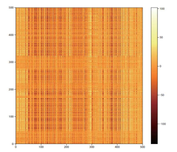
Fig. 5 Sample raster of edge connections for a typical video. Each video has 20 frames and 25 features per frame for a total of 500 features. Note that the rasters are asymmetric indicating that transfer between two nodes can have a directional dependence.
In this matrix the rows (and columns) are ordered as first by feature, 1-25, and then by frame, 1-20 (i.e., the first twenty-five rows, 0-24, correspond to the 25 features in the first frame, etc.). Thus, a periodic signature with length 25 might be expected but this does not appear. A Fourier transform of the data also does not show any periodic feature near length 25. In Fig. 6 we have taken the Fourier transform of each row of the video whose affinity matrix is shown in Fig. 5. These 500 transforms have then been averaged together to produce the displayed figure.
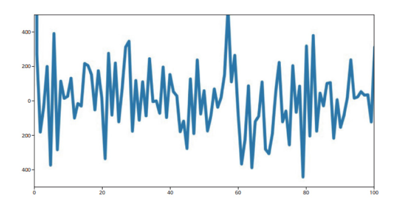
Fig. 6 Fourier transform of the edge connections in Fig. 5. Each row has been indiividually transformed and the results averaged together No significant periodicity at n=25 is discernable.
Clearly there is no distinct feature corresponding to a periodicity of 25. Indeed, the signature shows no prominent Fourier components at any length scale. Therefore, nodes in frames that are far separated are as likely to be joined by strong edges as nodes in neighboring frames or even the same frame. The implication here is that temporal proximity is not incorporated into the construction of the graph. All of the region features of all of the frames are included in the graph and no information is retained to indicate which notes are temporally close to which other nodes.
Also note in Fig. 5 that the edge strengths can be either positive or negative. This is not surprising in that the feature vectors themselves are not restricted to be positive definite but are rather arbitrary real vectors. Hence when the GCN process mixes feature vectors in a general linear combination it is sensible that the edges also are freely positive or negative.
It is possible to create a symmetrized version of the affinity matrix by using only the ϕ weights or the ϑ weights. In other words, we can write A(ri , rj) = wϕ(ri)∙wϕ(rj) and thereby expect A to be symmetric. Fig. 7 shows an example (the same video as in Fig. 5) of that symmetrized affinity matrix.
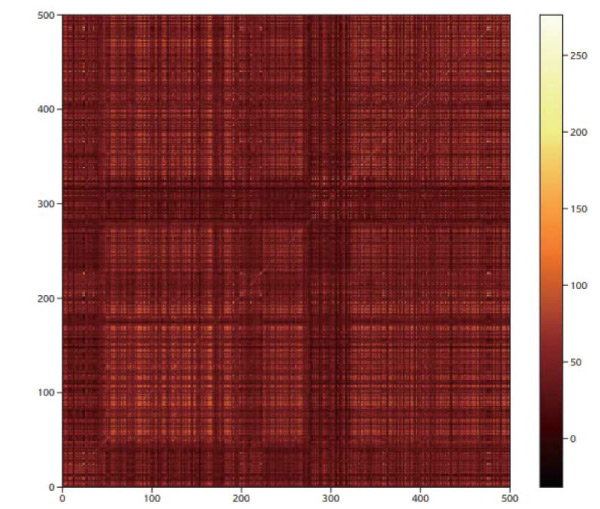
Fig. 7 Symmetrized version of video edge data from Fig. 5. Only one of the learned weight terms is included (see text). note that negative weights are significantly reduced but not eliminated altogether.
It is interesting that the symmetrized version of the affinity matrix shows significantly less – but not zero – likelihood for a weight to be negative.
4 Conclusion
In this short technical report, we have explored the detailed structure of a recently constructed deep learning model for matching videos with captions in the form of the MSR-VTT challenge. We have illustrated the architecture of the model and highlighted the video encoding side and in particular the novel technique of casting the features of the video in the form of a graph.
We have looked at the components of the graph which consist of feature vectors for nodes and a learned affinity matrix for edges. We have examined the structure and statistics of those edges showing a basic asymmetry in the raw weights and a type of “levelrepulsion” in the symmetrized version of the weights.
In the future we will look to correlate the properties of the learned edges with the specific nature of the features which lie at the nodes. In addition, as we discussed, we will determine how to include temporal correlations in property graph with the aim of increasing the accuracy of the captioning process.
5 Acknowledgements
The author would like to thank Prof. Raymond Fu and Mr. Chang Liu at Northeastern University for many discussions and Dr. Jun Amano for translating the abstract into Japanese.